When you are working in a spreadsheet and has lot many data, it is beneficial to format these types of data. The formatting is typically not applied by default, but you can always add them. For example, if you are interested in knowing all negative numbers of the spreadsheet, you can choose to display parentheses around negative numbers. Excel has a formatting option that automatically places parentheses which make it easier to locate.
Suppose you have a list of numbers that contains both positive and negative numbers and you want to put brackets around all negative numbers in the list. Just follow these steps to display parentheses around negative numbers in excel:
Step 1:
Open your file in Excel.
Step 2:
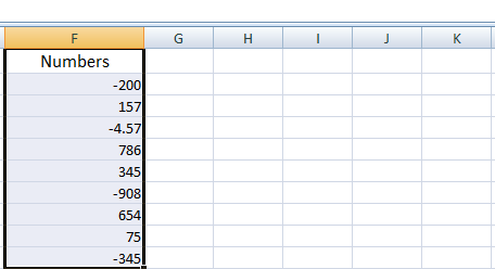
Now, select the cells to which to apply this formatting. Use your mouse to select the cells of the spreadsheet.
Step 3:
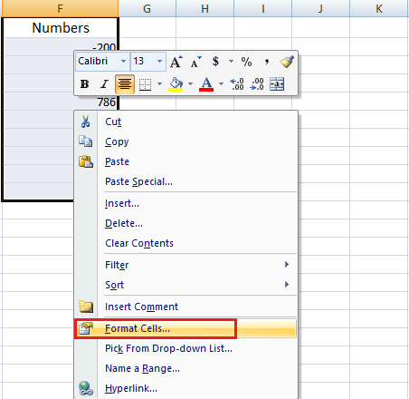
The next step is to right-click on one of the selected cells, and then click Format Cells option.
Step 4:
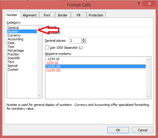
Click the Number or Currency option at the left side of the window.
Step 5:
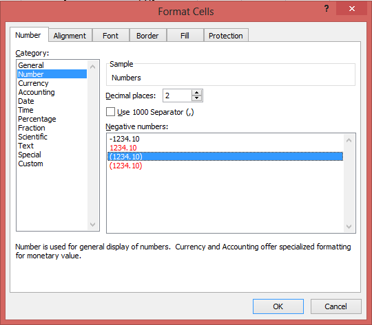
Click your preferred formatting option under Negative Numbers.
Step 6:
The next step is to click OK button at the bottom of the window to apply the changes.
Step 7:
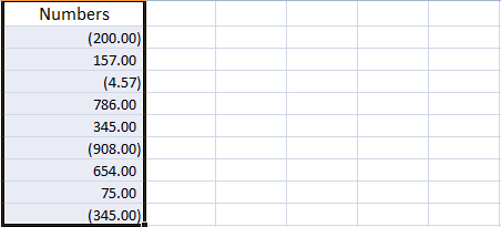
After applying the formatting, the numbers will be displayed automatically as shown in the image below.
If you are not able to right-click in the third step above, you can also access Format Cells window. Follow these steps to display parentheses around negative numbers:
Step 1:
Open your file in Excel.
Step 2:
Now, select the cells to which to apply this formatting. Use your mouse to select the cells of the spreadsheet.
Step 3:
Click on the Home tab on the top of the window and click Format button in the cells section and select format cells option.
Step 4:
Click the Number or Currency option at the left side of the window.
Step 5:
Click your preferred formatting option under Negative Numbers.
Step 6:
The next step is to click OK button at the bottom of the window to apply the changes.
Step 7:
After applying the formatting, the parentheses will be displayed automatically.
If you have any questions or queries, feel free to ask them in the comments. We would be more than happy to help you.
If you like our content, please consider sharing, leaving a comment or subscribing to our RSS feed to have future posts delivered to your feed reader.
Please follow us on twitter @CodeRewind and like us on facebook


