SmartArt includes special types of graphic objects that allow you to construct fancy graphical lists and diagrams in your spreadsheet. In Microsoft Excel, it is fairly simple to use SmartArt lists and diagrams. When you want to make visual representation of information, SmartArt is the apt tool. It enables you to combine your own text with predefined graphic shapes.
[leaderad]
Here are the steps to create SmartArt in Excel:
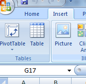
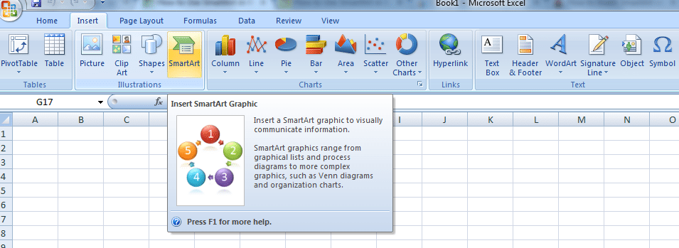
1) Open the spreadsheet in which you want to insert a SmartArt graphic. Go to Insert tab and click on SmartArt in the Illustrations Group.
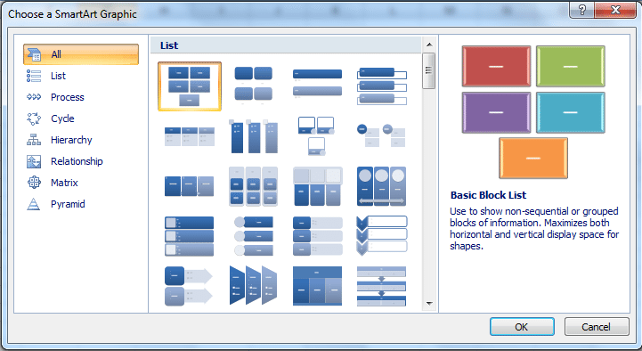
2) You will see many SmartArt graphics and you can choose the one that best suits your needs. You can choose categories from the left pane such as List, Process, Cycle, Hierarchy, Relationship, Picture and more. Click OK to insert graphical objects in your worksheet.
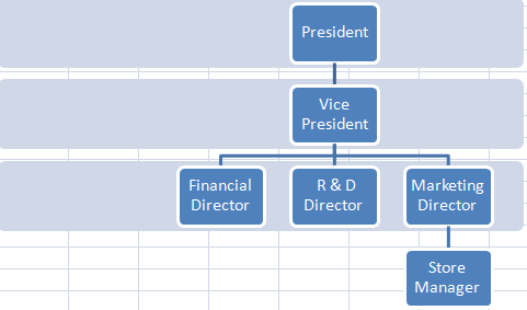
3) Excel inserts the basic structure of the list into your spreadsheet along with a text pane to its immediate left so that you can enter the text for the various parts of the diagram. An example is shown here:
4) You can format the text and graphics as per your choice. To format, select all the graphical objects that need same type of text formatting. Click on Commands buttons in the Font group on the Home tab of the Ribbon.
5) You can also use the Layouts, Change Colors, and SmartArt styles available in the Design tab of the SmartArt Tools. You can also choose colors by clicking Change Colors button in the SmartArt styles Group.
Some useful notes while creating SmartArt in Excel:
- When you enter text in the graphical objects, don’t press the Tab key or the Enter key to complete a text entry as you naturally do in a regular worksheet.
- When you finish entering text for the diagram, click the Close button on the text pane.
- You can delete the unused graphics by clicking them to select them and then, press Delete key.
If you want to suggest something on SmartArt in Excel, please feel free to share your thoughts in the comments section below!

